Estimating Pi
Implementation of Monte Carlo simulation to estimate the value of pi
In this notebook, we will estimate the value of $\pi$ using Monte Carlo simulation.
Monte Carlo simulation is a technique used to approximate the probability of an event by running the same simulation mutiple times and averaging the results [1].
For many years, people have known that there exists a constant called $\pi$ and were also aware of the fact that the circumference and the area of the circle with radius r, is 2.$\pi$.r and $\pi$.$r^2$, respectively. But what about the value of $\pi$?
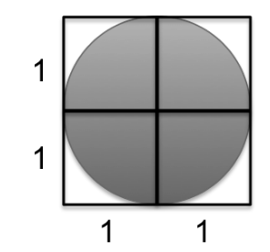
Two french mathematicians, Buffon and Laplace proposed to estimate the value of $\pi$ using stochastic simulation. They took a circle and inscribe it in a square with sides of length 2 units, so that the radius, r, of the circle is of length 1 (see figure below).

The area of circle is $\pi$.$r^2$ and since $r = 1$, $\pi = area$. This means that if we can figure out the area of circle, we can estimate the value of $\pi$.
To estimate the area of circle, Baffon suggested to drop a large number of needles in the vicinity of the square. The ratio of the number of needle tips lying within the square to the number of needle tips lying within the circle could then be used to estimate the area of the circle.
Now, if locations of needles are truly random, we can write:
$$\frac{\text{needles in circle}}{\text{needles in square}} = \frac{\text{area of circle}}{\text{area of square}}$$
We already know the area of square = 4, therefore, we can write:
$$\text{area of circle} = \frac{\text{4 * needles in circle}}{\text{needles in square}}$$
The only thing we need now is number of needles in circle and square. Lucky us, we have computers to simulate the dropping of needles. Unfortunately, computers were not a thing at Buffon's time so one has to try dropping a very large number of needles to get an approximation of $\pi$.
Code below estimates the value of $\pi$ using the Buffon-Laplace method. We will consider only the upper right-hand quadrant of the square.
import random
import numpy as np
import matplotlib.pyplot as plt


def getpi(numNeedles, numTrials):
  """ Calculates the value of pi for number of trails(numTrials) and number of needles(numNeedles).
  """

  estimates = []
  for trial in range(numTrials):
    inCircle = 0  # To count the number of needles that lie within the circle

    for needles in range(1, numNeedles + 1):
      x = random.random()
      y = random.random()

      # Needle will lie within the circle if and only if the distance from the origin is no greater than radius which is 1.
      if(x*x + y*y)**0.5 <= 1:
        inCircle +=1
    pi = 4*(inCircle/numNeedles)
    estimates.append(pi)
  stDev = np.std(estimates)
  curEst = sum(estimates)/len(estimates)
  print("Est. =", str(round(curEst, 5)), "Std. Dev =", str(round(stDev,5)), "Needles =", numNeedles)
# We increase the number of sample size i.e. number of needles after every 100 trials
Numneedles = [1000, 2000, 4000, 8000, 16000, 32000, 64000, 128000]
for i in Numneedles:
  getpi(i, 100)
One can see that the standard deviation decreases monotonically with the increase in the sample size i.e. number of needles. We also notice that the value of pi also improved steadily with increasing number of needles.
A more sophisticated version of this code can be found in [1] on Pg. 287.
Let me know if you have any comments or suggestions. Thanks for reading !
References:
[1] Introduction to Computation and Programming Using Python (with Application to Understanding Python), second edition, J.V. Guttag, MIT Press, 2016